Build compact collimators for high power LEDs
Introduction
The motion control system uses video surveillance of objects, which often requires additional lighting. Economical powerful LEDs work well with lighting in a wide viewing angle. To reduce the angle of illumination required collimator. The calculation of the collimating lenses may be made of, e.g., Zemax or Code V. For the calculation of complex collimators, containing reflectors, is a special environment, for example, LightTools or TracePro. In this work illustrates the structure and means of calculation of optimal collimators that reduce the viewing angle on the order of up to 10 degrees, also offered a manual version of the calculation.
the
Features of high power LEDs
High power LEDs have a wide viewing angle. Popular LEDs CREE is no exception. For example, the characteristics of the led XP-E2 [5].
• Size 3,45 x 3,45 x 2.08 mm
• Color: White
• Maximum current 1 a
• Maximum 3 watts
• The maximum luminous flux LM 283
• Nominal forward voltage of 2.9 V White @ 350 mA
• The maximum reverse voltage 5 V
• Viewing angle 110°
the
Collimators
There are many options of collimators, collecting divergent radiation in the surveillance zone. Among them are lenses (refracting light), reflectors and compound collimator consisting of lenses, refracting surfaces and reflectors (Fig. 1, Fig. 2).
The required uniform illumination of the object or a different distribution of light is achieved by using special materials, the scattering surfaces and the adjustment of the shapes of the elements of the collimator and their location.

Fig. 1. Examples of the structures of the collimator led [1,2,3,4].
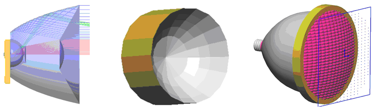
Fig. 2. Geometry demonstration environment models the design of optical devices LightTools.
the
Distribution of rays reflector
The profile of the reflectors is calculated from the angle and radiation pattern of the led, size of object and distance to it, and also required distribution of illumination of the object.
Some variants of distribution of rays of the led on the surface of the object shown in Fig. 3.
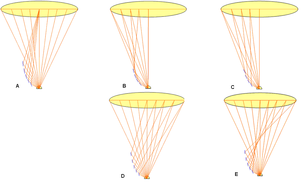
Fig. 3. The distribution of rays in the area of the object. A — focusing at the Central point; B, D — weak beams (see diagram) going to the periphery of the object, strong in the center (for increased intensity of the Central zone); options C and E collect the weak rays of in the center and strong at the periphery (for leveling the intensity of illumination).
the
Calculation profiles of the reflector
Calculation of the profile of the reflector focusing the rays from a point source (Fig. 3, variant a), can be performed without the use of special environments for the development of optical systems.
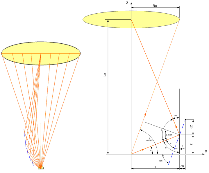
Fig. 4. The distribution of direct and the focused beams (in this figure, to the left, Fig. 3, option A) and diagram of the calculation of the profile of the reflector point source (right).
Further, the programs calculate and plot the profile of the reflector (Fig. 5) in the environment of MATLAB using the build Fig. 4.
the
clear all
% Initial DATA %%%%%%%%%%%%%%
Lo = 300; % distance to object in mm
Ro = 50/2; % radius of the object in mm

D_led = 3; % diameter in mm LED
Rt = 2; % Min radius of reflector >= D_led/2

dR = 0.0001; % step along X

if Rt < D_led/2
Rt = D_led/2
end
a_ini = 30; % angle in degree ini

% Calculation %%%%%%%%%%%%%%
a = pi*a_ini/180; % in rad

% Half field of view
a_max = pi/2-atan(Ro/Lo); % in rad

R(1) = Rt;
Z(1) = R(1) * tan(a);

f = pi/4;
i = 1;

while a < a_max && f > 0
ao = atan(Ro/(Lo-Z(i)));
b = pi/2 - a;
c_half = (pi - b - ao) / 2;
e = pi/2 - c_half;
f = b - e;
refl = pi/2 - f;

dZ = dR*tan(refl);

%next point
i = i+1;
R(i) = R(i-1) + dR;
Z(i) = Z(i-1) + dZ;
a = atan(Z(i)/R(i));
end

if 1
figure
plot(R,Z,'b')
grid
xlabel('Radius, mm');
ylabel('Length mm');
title(sprintf('FOV = %d deg',180-2*a_ini))
end
Diagram of calculation of the profile of the reflector (Fig. 3) is shown in Fig. 6.
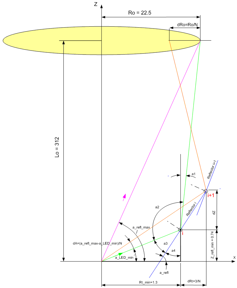
Fig. 6. Diagram of calculation of the profile of the reflector beams point of origin: "Weak" — the peripheral rays (radiation pattern of the led) go to the object boundaries, the Strong Central rays are collected in the center of the object (Fig. 3, option B).

Fig. 7. Profiles 6 mm reflectors (left) and angles of reflected rays (right). Here, the calculated angles relative to the plane of the source. So, angle 30 ° corresponds to the viewing angle is 120 = 2*(90-30). Accordingly, the minimum angle of direct rays (not on the reflector) is equal to 50°, as 2*(90 — 65о ).
Comparative profiles of the reflectors of options A,B,C,D,E (Fig. 3) is shown in Fig. 7. The maximum diameter of the reflectors is limited to 6 mm.
Comparison of profiles (Fig. 7) and distribution of rays (Fig. 3) shows that the length of the collimators and range of collected rays is maximal for options D and E. the E Collimator provides better uniformity of illumination of the object than the collimator In the Collimator D. has the greatest area for the placement of the lens that collects the rays are not hitting the reflector. The divergence angle of the direct rays passed inside of the reflector is 60 degrees (as 90-60*2).
the
Composite compact collimator
Composite collimator includes a reflector, of a limited size, and a lens that focuses the rays are not collected by the reflector. The software package LightTools or TracePro is used to calculate collimators with reflectors and lenses. The calculation of the lens can be performed separately, for example, Zemax or Code V.
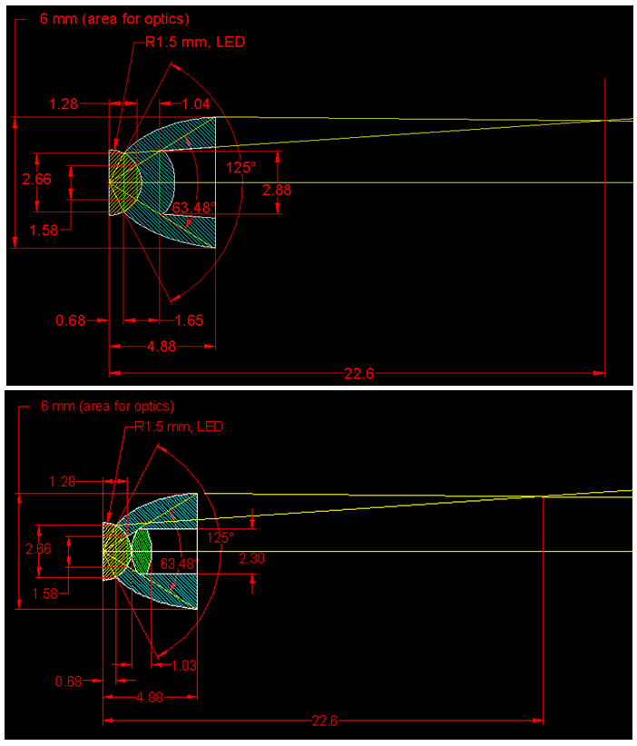
Fig. 8. Structure compact collimator organic glass PMMA (top) and a collimator with a glass lens made of glass BK7 (bottom) for the lighting of the 50 mm objects from a distance of 300 mm. the Calculation of the reflecting surface executed in MATLAB, to calculate the lens used the Zemax environment.
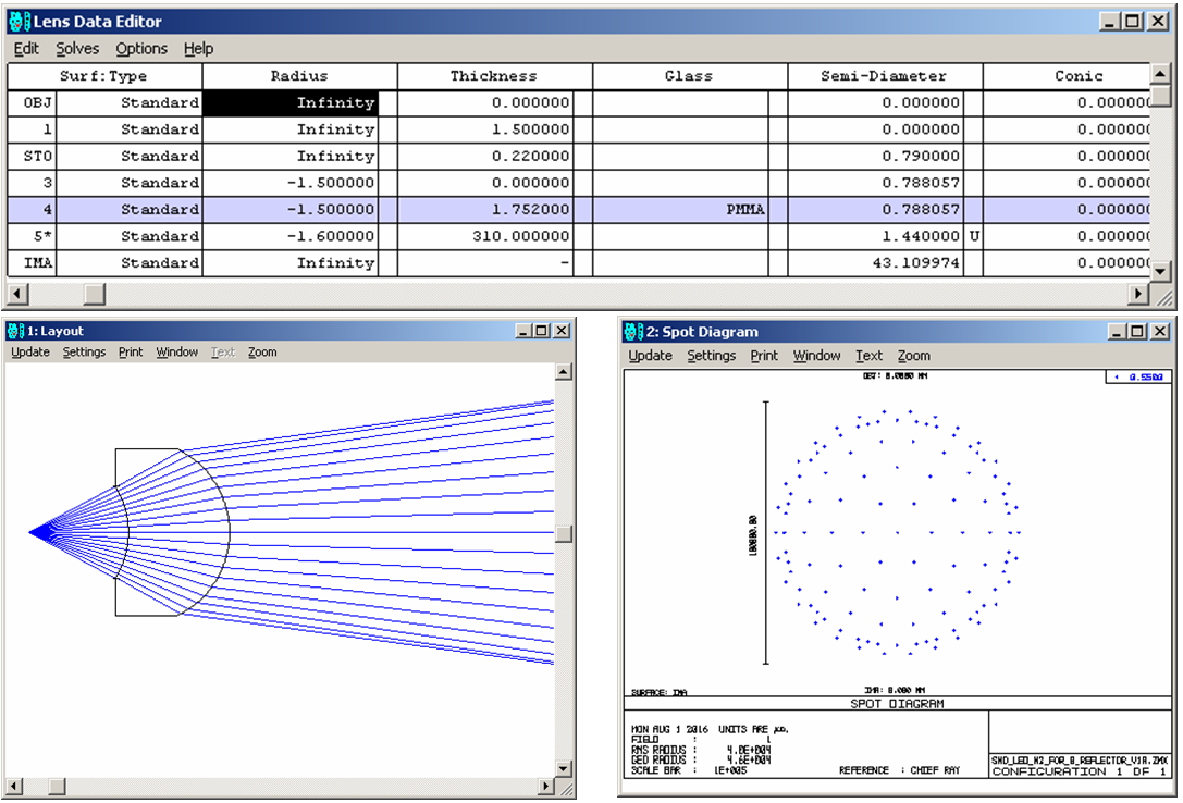
Fig. 9. The results of the calculation of the lens collimator of Fig. 8. in Zemax.
the
building a reflector in LightTools
The software package LightTools allows you to calculate the collimator and to optimize their parameters in automatic mode.
The results of the calculation in the environment LightTools optimal profile of the reflector without limiting its size to 50 mm lighting of the object remote from the led XP-E2 300 mm, shown in Fig. 10. The profile of the reflector described Bezier curve (Bezier) [6]. Model led XP-E2 taken from the library of LightTools. Optimal output diameter and length of the collimator amounted to 12.9 and 18.9 mm, respectively.
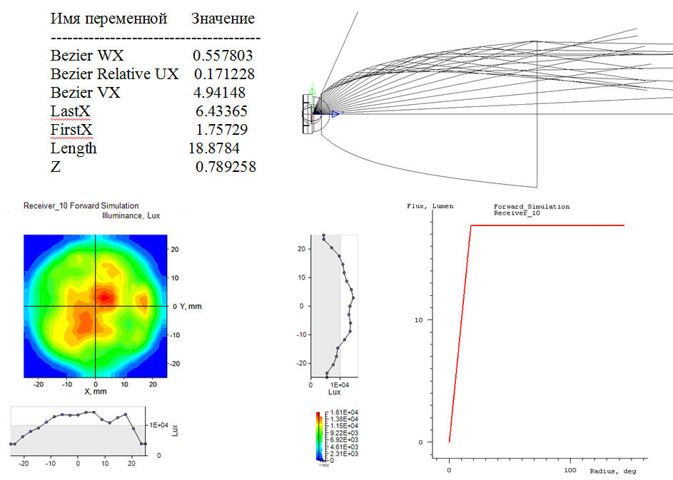
Fig. 10. The size and efficiency of the reflector 12.9 x 18.9 mm. Efficiency of 17.5% is determined by the ratio of the number of rays has reached the object to the number of rays emitted by the source.
The limitation of the diameter of the reflector 6.2 mm led to decrease of its efficiency from 17.5% to 5.6% (Fig. 11). This is due mainly to the fact that with the decrease in the area of reflection has increased the number of direct rays of the led within the area of the object.
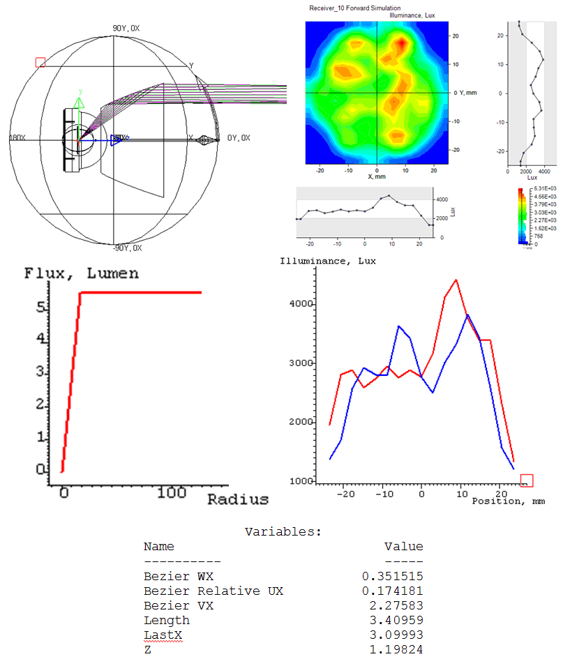
Fig. 11. Characteristics of light exposure and the setting of the optimum reflector for collecting rays led XP-E2 in the range of 69... 103 degrees. The maximum diameter of the reflector is limited to 6.2 mm. the Efficiency of a collimator of ~5.6 per cent.
The updated model is different from led point source because the radiation is formed by many point sources distributed over the entire surface of the diode, for example, in the area of 1 mm x 1 mm for the XP-E2. Viewing angles and polar patterns all sources are equal.
The profile of the reflector of radiation is a distributed source (Fig. 12) differs from the profile of the reflector for a localized source (Fig. 11), but their efficiency (~5.6%) of the same.
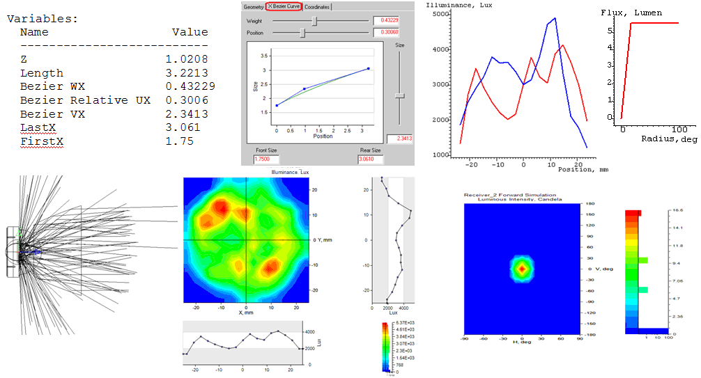
Fig. 12. The optimal parameters LightTools reflector of radiation is a distributed source XP-E2. The maximum diameter of the reflector is limited to 6.2 mm. the Efficiency of a collimator of ~5.6 percent.
the
comparing the profiles of the reflectors are calculated in MATLAB and LightTools
The profiles of the reflectors shown in Fig. 13, designed in MATLAB (profiles: A,B,C,D,E) and LightTools (profiles: point LT, LT dist, LT unlim). In MATLAB performed a manual calculation for point sources. In LightTools optimization profiles performed in the automatic mode for point and distributed sources with the restriction (6.2 mm) and without limiting the diameter of the reflector for uniform illumination of 50 mm of the object remote from the source 310 mm.
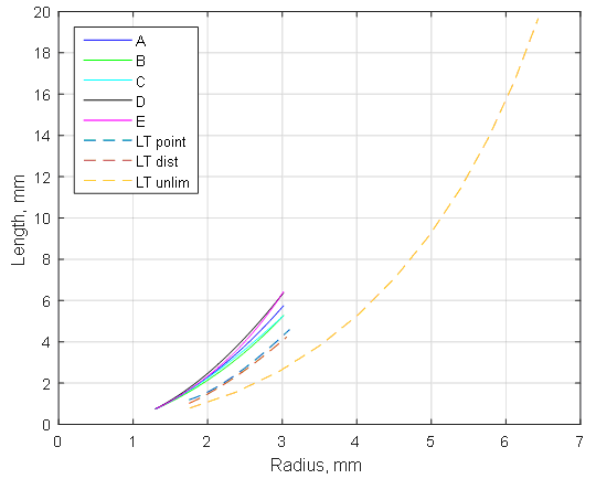
Fig. 13. The profiles of the reflectors A, B, C, D, E, of limited diameter (6 mm), calculated in MATLAB for point source; point LT — limited diameter (6.2 mm) obtained in LightTools for a point source; LT dist, of limited diameter (6.2 mm) obtained in LightTools distributed source; LT unlim — free size, designed in LightTools for a point source.
Optimization algorithms parameters in LightTools hidden from the user. To understand the LightTools optimization algorithm, which was used in the calculation of type "LT dist" (Fig. 13) the distribution of beams in MATLAB (Fig. 14).
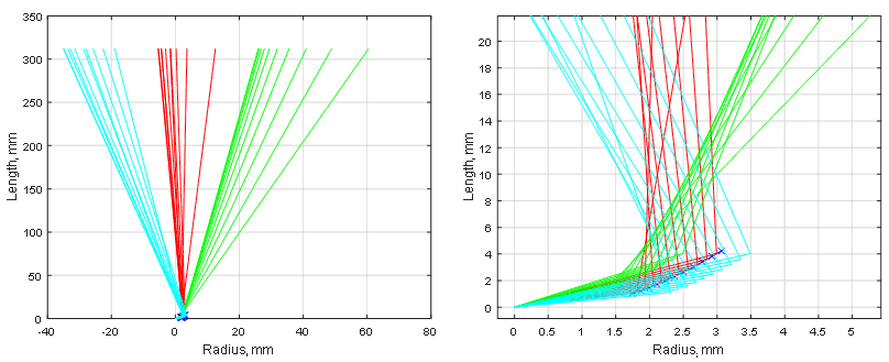
Fig. 14. The course of the rays of the distributed source is reflected to a zone of 50 mm from a distance of 310 mm, the diagram (left) and enlarged detail (right). Considers the radiation from the edges (blue and green lines) and the center (red lines) distributed source. Separation of regional and Central beams 1x1 mm source is achieved by displacement of the reflector by ±0.5 mm.
The distribution of the rays (Fig. 14) shows that the optimization LightTools found the profile of the reflector for the Central point source illumination 1/3 area of the object and used this profile to illuminate the entire area of the object radiation source distributed on a square of 1x1 mm led
Code MATLAB to compute the array of points of the optimal profile of the reflector — bézier curve ('Besier_profile_dist_source.mat'), given parameters LightTools Bezier_WX Bezier_Relative_UX and Bezier_VX:
the
% A quadratic Bezier curve is the path traced by the function B(t),
% given points P0, P1, and P2,
% B(t) = (1 - t)[(1 - t)P0 + t P1] + t[(1 - t)P1 + t P2],
% 0 <= t <= 1

Bezier_WX = 0.43229;
Bezier_Relative_UX = 0.3006;
Bezier_VX = 2.3413;

Front_Size = 1.75;
Rear_Size = 3.061;
Length = 3.2213;
Z = 1.0208;

LastX = Rear_Size;

Px = [Z, Z+Length*Bezier_Relative_UX Z+Length];
Py = [Front_Size Bezier_VX LastX];

i = 0;
for t = 0:0.1:1
i = i+1;
bx_t(i) = (1-t)^2*Px(1) + 2*t*(1-t)*Px(2) + t^2*Px(3);
by_t(i) = (1-t)^2*Py(1) + 2*t*(1-t)*Py(2) + t^2*Py(3);
end

save('Besier_profile_dist_source','bx_t','by_t')

MATLAB code for constructing the Central beam Fig. 14:
load('Besier_profile_dist_source')
offset = 0.5;

X_base = by_t; Y = bx_t;


X_left = by_t - offset;
X_right = by_t + offset;
clear by_t bx_t;

% CENTER
dYdX = diff(Y)./diff(X_base);
a_refl=(180/pi).*atan(dYdX);

for i = 1:length(X_base)-1
p_x(i) = (X_base(i+1)+X_base(i))/2;
p_y(i) = Y(i)+ dYdX(i)*((X_base(i+1)-X_base(i))/2);
end

a_LED =(180/pi).*atan(p_y./p_x);
a_out = 2.*a_refl - a_LED;
X_t = p_x + (312-p_y)./tan(a_out.*(pi/180));


% plotting
figure
plot(X_base,Y,'b')
hold on
plot(X_base,Y,'xb')
hold on
for i = 1:length(p_x)
plot([0 p_x(i)],[0 p_y(i)],'r')
hold on
plot([p_x(i) X_t(i)],[p_y(i), 312],'r')
hold on
end
%  end  of plotting
the
Manual calculation of collimator
To perform manual calculations and the reflector of the distributed source must:
1. Find the coordinates of the reflector closest to the source.
2. To calculate the profile of the reflector (see the algorithm section the Calculation of the profiles of the reflector) for a reduced area of the object, for example, 1/3.
Through the starting point of the reflector nearest the source should pass the beams emitted by all points in the plane of the led. The direct rays passing through the starting point should illuminate the area commensurate with the object at the desired distance from the source.
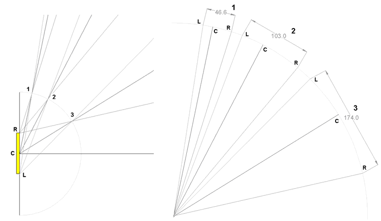
Fig. 15. The construction of beams to find the start point of the reflector. Zones are located on a circle with a radius of 310 mm (right figure) equal to the distance to the object. The left figure is the magnified image with the led surface with a radius of 1.5 mm.
The position of the initial point of the reflector corresponds to the point 1 on the surface of the led with a radius of 1.5 mm (Fig. 15) through which extreme (L and R) and the Central © the rays distributed emitter in a zone about 50 mm, separated from the source 310 mm.
The angle of the calculated collimator with a reflector can be reduced, enabling the structure of the collimator lens, as shown in Fig. 8.
references
1. Collimation lens system for LED. Patent US 7580192 B1.
2. LED collimation optics with improved performance and reduced size www.google.com/patents/US6547423
3. RXI LED collimator needs no metalization www.laserfocusworld.com/articles/2012/01/rxi-led-collimator-needs-no-metalization.html
4. LED OPTICS: Efficient LED collimators have simple designhttp://www.laserfocusworld.com/articles/print/volume-48/issue-06/world-news/efficient-led-collimators-have-simple-design.html
5. Delivering high performance and lower system cost to XLamp XP LED designs www.cree.com/LED-Components-and-Modules/Products/XLamp/Discrete-Directional/XLamp-XPE2
6. Wikipedia. Bézier, Pierre ru.wikipedia.org/wiki/%D0%91%D0%B5%D0%B7%D1%8C%D0%B5,_%D0%9F%D1%8C%D0%B5%D1%80
7. Dr. Bob Davidov. Build perfect optics in Zemax. portalnp.ru/wp-content/uploads/2016/07/4.7_Paraxial_Optics_Design_in_Zemax_1a.pdf
8. Dr. Bob Davidov. Computer management technologies in technical systems. portalnp.ru/author/bobdavidov


Комментарии
Отправить комментарий