Z-order vs R-tree, optimization and 3D

Previously (1, 2) we have substantiated and demonstrated the possibility of the existence
a spatial index that has all of the advantages of a conventional B-Tree index and
not inferior in performance index based on R-Tree.
Under the cut is a generalization of the algorithm for three-dimensional space, optimization and benchmarks.

3D

Why do I need this 3D? The fact that we live in a three dimensional world. Therefore, the data are either in geo-coordinates (latitude, longitude) and then the more distorted the farther they are from the equator. Or attached a projection, which is adequate only for a certain space of these coordinates. A three-dimensional index allows you to place points on the sphere and to avoid the material misstatement. To obtain the search extent sufficient to define a sphere center of the desired cube and retreat to the side all coordinates on radius.

Fundamentally three-dimensional version of the algorithm does not differ from two-dimensional — the only difference in working with key:
the

alternation of bits in the key is now 3 steps instead of 2 ie ...z1y1x1z0y0x0
key is now 96, and not 64 bits. Option to place all the 64-bit key is rejected because it gives a total of 21 discharge to coordinate, that would make us a bit constrained. Also coming 4 and 6 dimensional keys (guess why), and there is not enough 64 did, so why delay the inevitable. Fortunately, it is not so difficult
therefore, the key now is not bigint, and numeric and key interface methods will be needed for translation from numeric and back
change the method of obtaining the key from the coordinates and back
and the method of splitting of the subquery. Recall, for splitting a query that is represented by two keys corresponding to left bottom and right upper corners we:
- found in them the most distinguished senior bit m
- the upper-right corner of the smaller of the new subquery is obtained by setting to 1 all the bits corresponding to the coordinates of m under m
- bottom left corner more of the new subquery is obtained by setting to 0 all bits of the respective m the coordinates of m under the
in Fact, nothing has changed, just the level one coordinates to go with other step

Numeric

Numeric us itself is not directly accessible from the extension. You have to use a universal mechanism for calling functions with marshalling — DirectFunctionCall[X] ‘include/fmgr.h’, where X is the number of arguments.

Inside is arranged as a numeric array short, each containing 4 decimal numbers from 0 to 9999. In its interface there is no shifts or division with the return of the module. As well as special functions for working with degrees 2 (with this device, they are out of place). Therefore, to parse numeric two int64 is necessary to act so:
the

void bit3Key_fromLong(bitKey_t *pk Datum dt)
{
Datum divisor_numeric;
Datum divisor_int64;
Datum low_result;
Datum upper_result;

divisor_int64 = Int64GetDatum((int64) (1ULL << 48));
divisor_numeric = DirectFunctionCall1(int8_numeric, divisor_int64);

low_result = DirectFunctionCall2(numeric_mod, dt, divisor_numeric);
upper_result = DirectFunctionCall2(numeric_div_trunc, dt, divisor_numeric);
pk- > vals_[0] = DatumGetInt64(DirectFunctionCall1(numeric_int8, low_result));
pk- > vals_[1] = DatumGetInt64(DirectFunctionCall1(numeric_int8, upper_result));
pk- > vals_[0] |= (pk- > vals_[1] & 0xffff) << 48;
pk- > vals_[1] >>= 16;
}

And for the inverse transform, as follows:
the

Datum bit3Key_toLong(const bitKey_t *pk)
{
uint64 lo = pk- > vals_[0] &0xffffffffffff;
uint64 hi = (pk- > vals_[0] >> 48) | (pk- > vals_[1] << 16);
uint64 mul = 1ULL << 48;
Low_result Datum = DirectFunctionCall1(int8_numeric, Int64GetDatum(lo));
Upper_result Datum = DirectFunctionCall1(int8_numeric, Int64GetDatum(hi));
Mul_result Datum = DirectFunctionCall1(int8_numeric, Int64GetDatum(mul));
Datum nm = DirectFunctionCall2(numeric_mul, mul_result, upper_result);
return DirectFunctionCall2(numeric_add, nm, low_result);
}

Working with arbitrary precision arithmetic generally a thing not fast, especially when it comes to divisions. Therefore, the author has an overwhelming desire to ‘hack’ numeric and parse it yourself. Had to duplicate locally the definitions of numeric.c and process raw short s. It was easy and accelerated performance.

Solid subqueries.

As we know, the algorithm splits the subquery as long as the underlying data will not completely fit on a single disk page. Here's how:

at the entrance of a subquery, it has a range of values between the left bottom (middle) and upper right (far) corners. Coordinates became more, but the essence is the same
do a search in a BTree keyed to the smaller angle
get up at the same leaf page and check the last value
if the last value >= the key value of the larger angle, scan the entire page and recorded the results all came in search extent
if less, continue to break down the request

However, it may happen that a subquery, the data for which are contained in dozens or hundreds of pages is entirely contained within the original search extent. There is no point in cutting it further, data from the interval you can safely without any checks to make to the result.

How can one recognize such a subquery? Quite simple —
the

its dimensions along all coordinates should be in degrees and is equal to 2 (cube)
the angles must lie on the corresponding lattice with a pitch in the same level 2

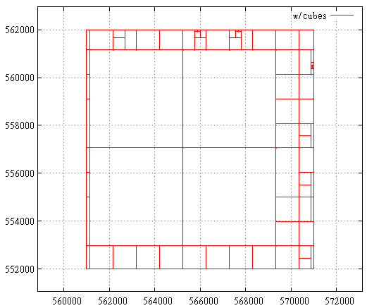
Here is a map of subqueries before optimization cubes:

And here is after:

Benchmark

In table are summarized the comparative results of the original algorithm, optimized version and GiST R-Tree.
R-Tree is two-dimensional for comparison, the z-index made the pseudo-3D data, i.e., (x, 0, z). From the point of view of the algorithm there is no difference, we're just giving R-tree some odds.

Data — 100 000 000 random points in the [0...1 000 000, 0...0, 0...1 000 000].

The measurements were carried out on a modest virtual machine with two cores and 4 GB of RAM, so the times are not absolute values, but the numbers of pages read is still possible to trust.
The times shown in the second runs, on a heated server and virtual machine. The number of read buffers — into the fresh-raised server.
the the the the the the the the

Npoints	Nreq	Type	Time(ms)	Reads	Hits
1	100 000	old new rtree	.37 .36 .38	1.13154 1.13307 1.83092	3.90815 3.89143 3.84164
10	100 000	old new rtree	.40 .38 .46	1.55 1.57692 2.73515	8.26421 7.96261 4.35017
100	100 000	old new rtree(*)	.63 .48 .50 ... 7.1	3.16749 3.30305 6.2594	45.598 31.0239 4.9118
1 000	100 000	old new rtree(*)	2.7 1.2 1.1 ... 16	11.0775 13.0646 24.38	381.854 165.853 7.89025
10 000	10 000	old new rtree(*)	22.3 5.5 4.2 ... 135	59.1605 65.1069 150.579	3606.73 651.405 27.2181
100 000	10 000	old new rtree(*)	199 53.3 35...1200	430.012 442.628 1243.64	34835.1 2198.11 186.457
1 000 000	1 000	old new rtree(*)	2550 390 300 ... 10000	3523.11 3629.49 11394	322776 6792.26 3175.36

where
Npoints — the average number of points in the results
Nreq — the number of queries in the series
Type — ‘old’ — original version
‘new’ — optimize numeric and continuous subqueries;
’rtree’- gist only 2D rtree,
(*) — in order to compare search time,
had to reduce the series 10 times,
otherwise, the page does not fit into the cache
Time(ms) — average time of query execution
Reads — the average number of readings by request
Hits — the number of accesses to the buffers
In graphs this data looks like this:

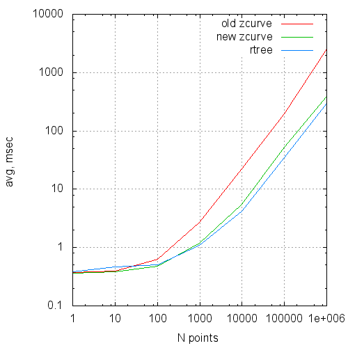
The average query time to the size of the request

The average number of reads in the query from the request size.

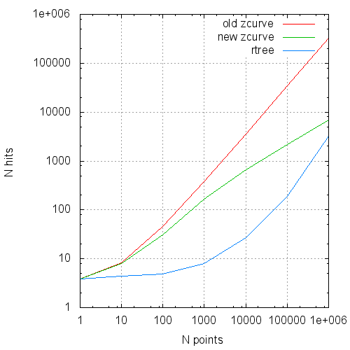
The average number of cache pages to the request from the request size.

Conclusions

So far so good. Continue to move in the direction of use for the spatial index Hilbert curve, as well as complete measurements on non-synthetic data.

PS: describes the changes is available here.

Article based on information from habrahabr.ru

Поиск по этому блогу

computer express